Using Random Forest to Predict Customer Churn

Junior Data Scientist Job simulation at Boston Consulting Group (BCG), using feature engineering and machine learning models to determine the influence of price sensitivity on custormer churn.
Price sensitivity is the degree to which demand changes when the cost of energy (electricity and gas) changes. ~ PowerCo.
Complete Project repository:

- Business understanding & Problem framing
- Exploratory data analysis & data cleaning
- Feature engineering & Hypothesis framing
- Modelling and evaluation
- Insights & Recommendations
Business understanding & Problem framing
Our client PowerCo - a major gas and electricity utility that supplies to small and medium sized enterprises is concerned about their customers leaving for better offers from other energy providers (customer churn). The energy market has had a lot of change in recent years nd there are now more options than ever for customers to choose from. They would like to diagnose the the reason why their customers are churning. One of the leading objective is - How sensitive are PowerCo customers to pricing and how does it influence the customer’s decision stay or leave PowerCo.
Data required;
- Customer data - historical electricity and gas consumption, date customer joined (subscribed for services)
- Churn data - indicating if customer churned or not (reclassified as 1 nad 0)
- Historical and seasonal pricing data - the price the client charges its customers and how it changes with demand.
Work Plan;
In order to test the hypothesis of how pricing affects churn, we defined what data we need from PowerCo, and what variables best define price sensitivity, prepare the data and engineer features. A binary classificantion model was used and trained to extrapolate the extent to which price sensitivity influences churn.
Exploratory data analysis & data cleaning
Data Overview
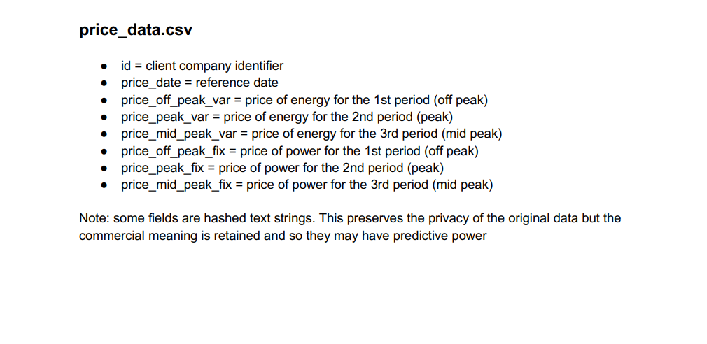
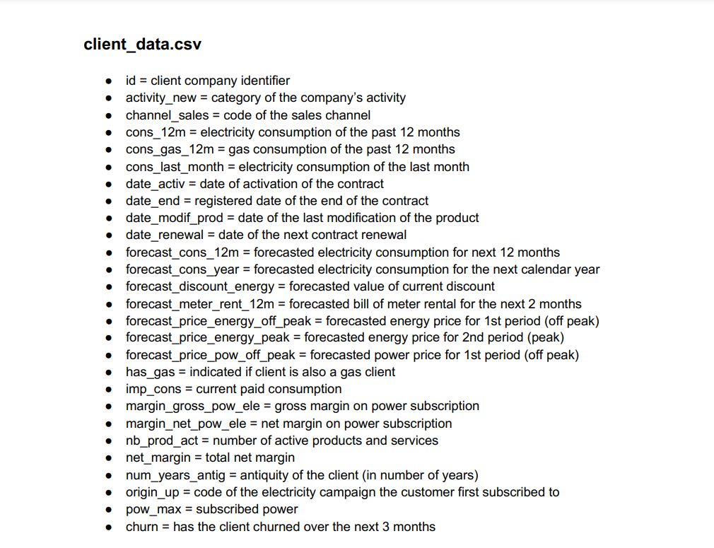
Data Import
import matplotlib.pyplot as plt
import seaborn as sns
import pandas as pd
import numpy as np

# Shows plots in jupyter notebook
%matplotlib inline

# Set plot style
sns.set(color_codes=True)

client_df = pd.read_csv('client_data.csv')
price_df = pd.read_csv('price_data.csv')
For modelling purposes we convert columns into date time
client_df['date_activ'] = pd.to_datetime( client_df['date_activ'])
client_df['date_end'] = pd.to_datetime( client_df['date_end'])
client_df['date_modif_prod'] = pd.to_datetime( client_df['date_modif_prod'])
client_df['date_renewal'] = pd.to_datetime( client_df['date_renewal'])
client_df.head(3)
It is useful to first understand the data that you’re dealing with along with the data types of each column and na values in those columns. The data types may dictate how you transform and engineer features.
# Check for column data types
print(client_df.info())
print(price_df.info())

#Check for missing values in columns
print(client_df.isna().sum())
print(price_df.isna().sum())
Descriptive statistics
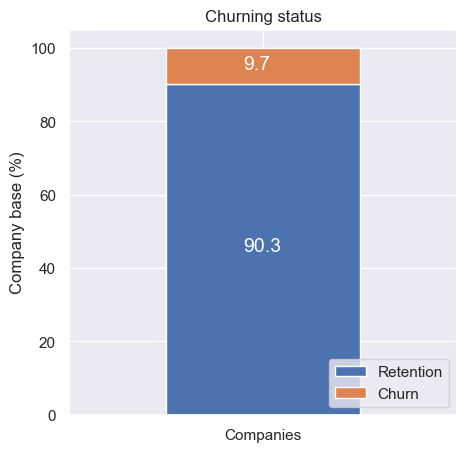
To visualise the statistics of churned customers, we used function ‘plot_stacked_bars’. The code below shows that close to 10% of PowerCo customers churned in the last three months
churn = client_df[['id', 'churn']]
churn.columns = ['Companies', 'churn']
churn_total = churn.groupby(churn['churn']).count()
churn_percentage = churn_total / churn_total.sum() * 100
plot_stacked_bars(churn_percentage.transpose(), "Churning status", (5, 5), legend_="lower right")
Complete exploratory data analysis script -
Feature engineering & Hypothesis framing
Hypothesis 1: “The difference between off-peak prices in December and January the preceding year could be a significant feature when predicting customer churn”
Load cleaned data set after EDA
df = pd.read_csv('C:/Users/farie/Downloads/clean_data_after_eda.csv')
df["date_activ"] = pd.to_datetime(df["date_activ"], format='%Y-%m-%d')
df["date_end"] = pd.to_datetime(df["date_end"], format='%Y-%m-%d')
df["date_modif_prod"] = pd.to_datetime(df["date_modif_prod"], format='%Y-%m-%d')
df["date_renewal"] = pd.to_datetime(df["date_renewal"], format='%Y-%m-%d')
Calculate the difference between off-peak prices in December and preceding January
price_df = pd.read_csv('price_data.csv')
price_df["price_date"] = pd.to_datetime(price_df["price_date"], format='%Y-%m-%d')
price_df.head()

# Group off-peak prices by companies and month
monthly_price_by_id = price_df.groupby(['id', 'price_date']).agg({'price_off_peak_var': 'mean', 'price_off_peak_fix': 'mean'}).reset_index()

# Get january and december prices
jan_prices = monthly_price_by_id.groupby('id').first().reset_index()
dec_prices = monthly_price_by_id.groupby('id').last().reset_index()

# Calculate the difference
diff = pd.merge(dec_prices.rename(columns={'price_off_peak_var': 'dec_1', 'price_off_peak_fix': 'dec_2'}), jan_prices.drop(columns='price_date'), on='id')
diff['offpeak_diff_dec_january_energy'] = diff['dec_1'] - diff['price_off_peak_var']
diff['offpeak_diff_dec_january_power'] = diff['dec_2'] - diff['price_off_peak_fix']
diff = diff[['id', 'offpeak_diff_dec_january_energy','offpeak_diff_dec_january_power']]

#merger files
df = pd.merge(df, diff, on='id')
df.head()
Hypothesis 2: “Average and max price changes between periods (peak and low season) through out the entire year could be a significant feature when predicting customer churn”
mean_prices = price_df.groupby(['id']).agg({
    'price_off_peak_var': 'mean',
    'price_peak_var': 'mean',
    'price_mid_peak_var': 'mean',
    'price_off_peak_fix': 'mean',
    'price_peak_fix': 'mean',
    'price_mid_peak_fix': 'mean'
}).reset_index()

# Calculate the mean difference between consecutive periods
mean_prices['off_peak_peak_var_mean_diff'] = mean_prices['price_off_peak_var'] - mean_prices['price_peak_var']
mean_prices['peak_mid_peak_var_mean_diff'] = mean_prices['price_peak_var'] - mean_prices['price_mid_peak_var']
mean_prices['off_peak_mid_peak_var_mean_diff'] = mean_prices['price_off_peak_var'] - mean_prices['price_mid_peak_var']
mean_prices['off_peak_peak_fix_mean_diff'] = mean_prices['price_off_peak_fix'] - mean_prices['price_peak_fix']
mean_prices['peak_mid_peak_fix_mean_diff'] = mean_prices['price_peak_fix'] - mean_prices['price_mid_peak_fix']
mean_prices['off_peak_mid_peak_fix_mean_diff'] = mean_prices['price_off_peak_fix'] - mean_prices['price_mid_peak_fix']

columns = [
    'id',
    'off_peak_peak_var_mean_diff',
    'peak_mid_peak_var_mean_diff',
    'off_peak_mid_peak_var_mean_diff',
    'off_peak_peak_fix_mean_diff',
    'peak_mid_peak_fix_mean_diff',
    'off_peak_mid_peak_fix_mean_diff'
]
df = pd.merge(df, mean_prices[columns], on='id')
Hypothesis 3: “How long a company has been a client of PowerCo (tenure) could be a significant feature when predicting customer churn”
- months_activ = Number of months active until reference date (Jan 2016)
- months_to_end = Number of months of the contract left until reference date (Jan 2016)
- months_modif_prod = Number of months since last modification until reference date (Jan 2016)
- months_renewal = Number of months since last renewal until reference date (Jan 2016)
def convert_months(reference_date, df, column):
    """
    Input a column with timedeltas and return months
    """
    time_delta = reference_date - df[column]
    months = (time_delta / np.timedelta64(1, 'M')).astype(int)
    return months

# Create reference date
reference_date = datetime(2016, 1, 1)

# Create columns
df['months_activ'] = convert_months(reference_date, df, 'date_activ')
df['months_to_end'] = -convert_months(reference_date, df, 'date_end')
df['months_modif_prod'] = convert_months(reference_date, df, 'date_modif_prod')
df['months_renewal'] = convert_months(reference_date, df, 'date_renewal')
Transform categorical data using one hot encoding (dummy variables)
df = pd.get_dummies(df, columns=['channel_sales'], prefix='channel')
df = pd.get_dummies(df, columns=['origin_up'], prefix='origin_up')
Transforming numerical data to remove the effect of skewed distribtion and also improve the speed at which predictive models are able to converge to its best solution. Note: We cannot apply log to a value of 0, so we will add a constant of 1 to all the values
# Apply log10 transformation
df["cons_12m"] = np.log10(df["cons_12m"] + 1)
df["cons_gas_12m"] = np.log10(df["cons_gas_12m"] + 1)
df["cons_last_month"] = np.log10(df["cons_last_month"] + 1)
df["forecast_cons_12m"] = np.log10(df["forecast_cons_12m"] + 1)
df["forecast_cons_year"] = np.log10(df["forecast_cons_year"] + 1)
df["forecast_meter_rent_12m"] = np.log10(df["forecast_meter_rent_12m"] + 1)
df["imp_cons"] = np.log10(df["imp_cons"] + 1)
Complete feature engineering script -
Modelling and evaluation
###Import packages for modelling
import warnings
warnings.filterwarnings("ignore", category=FutureWarning)

from sklearn import metrics
from sklearn.model_selection import train_test_split
from sklearn.ensemble import RandomForestClassifier
Splitting the dataset into training and test samples
# Make a copy of our data
train_df = df.copy()

# Separate target variable from independent variables
y = df['churn']
X = df.drop(columns=['id', 'churn'])
print(X.shape)
print(y.shape)

X_train, X_test, y_train, y_test = train_test_split(X, y, test_size=0.25, random_state=42)
print(X_train.shape)
print(y_train.shape)
print(X_test.shape)
print(y_test.shape)
Model Training
- We use a Random Forest Classifier whixh is an ensemble algorithm
- We add a randomsearch CV which helps fine tune the optimal parameters
- To make random forest more suitable for learning from extremely imbalanced data (only 9% of churned customers in dataset) follows the idea of cost sensitive learning. Since the RF classifier tends to be biased towards the majority class, we placed a heavier penalty on misclassifying the minority class (class_weight = ‘balanced’)
rf = RandomForestClassifier(random_state = 42)#run model

from pprint import pprint #to print parameters used by model
# Look at parameters used by our current forest
print('Parameters currently in use:\n')
pprint(rf.get_params())

#select the optimal parameters
from scipy.stats import randint

rs_space={'max_depth':list(np.arange(10, 100, step=10)) + [None],
              'n_estimators':np.arange(10, 1000, step=50),
              'max_features':randint(1,7),
              'criterion':['gini','entropy'],
              'min_samples_leaf':randint(1,4),
              'min_samples_split':np.arange(2, 10, step=2)
         }


from sklearn.model_selection import RandomizedSearchCV

rf = RandomForestClassifier(random_state = 42, class_weight="balanced_subsample")#run model, but we add class weight because there ins an imbalance in values between class of independent variable
rf_random = RandomizedSearchCV(rf, rs_space, n_iter=500, scoring='accuracy', n_jobs=-1, cv=3)
model_random = rf_random.fit(X_train,y_train)
Model Evaluation
#check model performance
print("tuned hpyerparameters :(best parameters) ",model_random.best_params_)
print("accuracy :",model_random.best_score_)

##evaluate model with test data
evaluator(model_random,X_test,y_test)
y_pred = model_random.predict(X_test)
plot_confusion_matrix(y_test, y_pred)
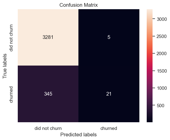
True positives: 21
False positives: 5
True negatives: 3281
False negatives: 345

Accuracy: 90%
Precision: 82%
Recall: 5%
Looking at these results there are a few things to point out:
- Within the test set about 10% of the rows are churners (churn = 1).
- Looking at the true negatives, we have 3281 out of 3286. This means that out of all the negative cases (churn = 0), we predicted 3282 as negative (hence the name True negative). This is great!
- Looking at the false negatives, this is where we have predicted a client to not churn (churn = 0) when in fact they did churn (churn = 1). This number is quite high at 345, we want to get the false negatives to as close to 0 as we can, so this would need to be addressed when improving the model.
- Looking at false positives, this is where we have predicted a client to churn when they actually didnt churn. For this value we can see there are 5 cases, which is great!
- With the true positives, we can see that in total we have 366 clients that churned in the test dataset. However, we are only able to correctly identify 21 of those 366, which is very poor.
- Looking at the accuracy score, this is very misleading! Hence the use of precision and recall is important. The accuracy score is high, but it does not tell us the whole story.
- Looking at the precision score, this shows us a score of 0.82 which is not bad, but could be improved.
- However, the recall shows us that the classifier has a very poor ability to identify positive samples. This would be the main concern for improving this model!
So overall, we’re able to very accurately identify clients that do not churn, but we are not able to predict cases where clients do churn! What we are seeing is that a high % of clients are being identified as not churning when they should be identified as churning. This in turn tells me that the current set of features are not discriminative enough to clearly distinguish between churners and non-churners.
Model understanding
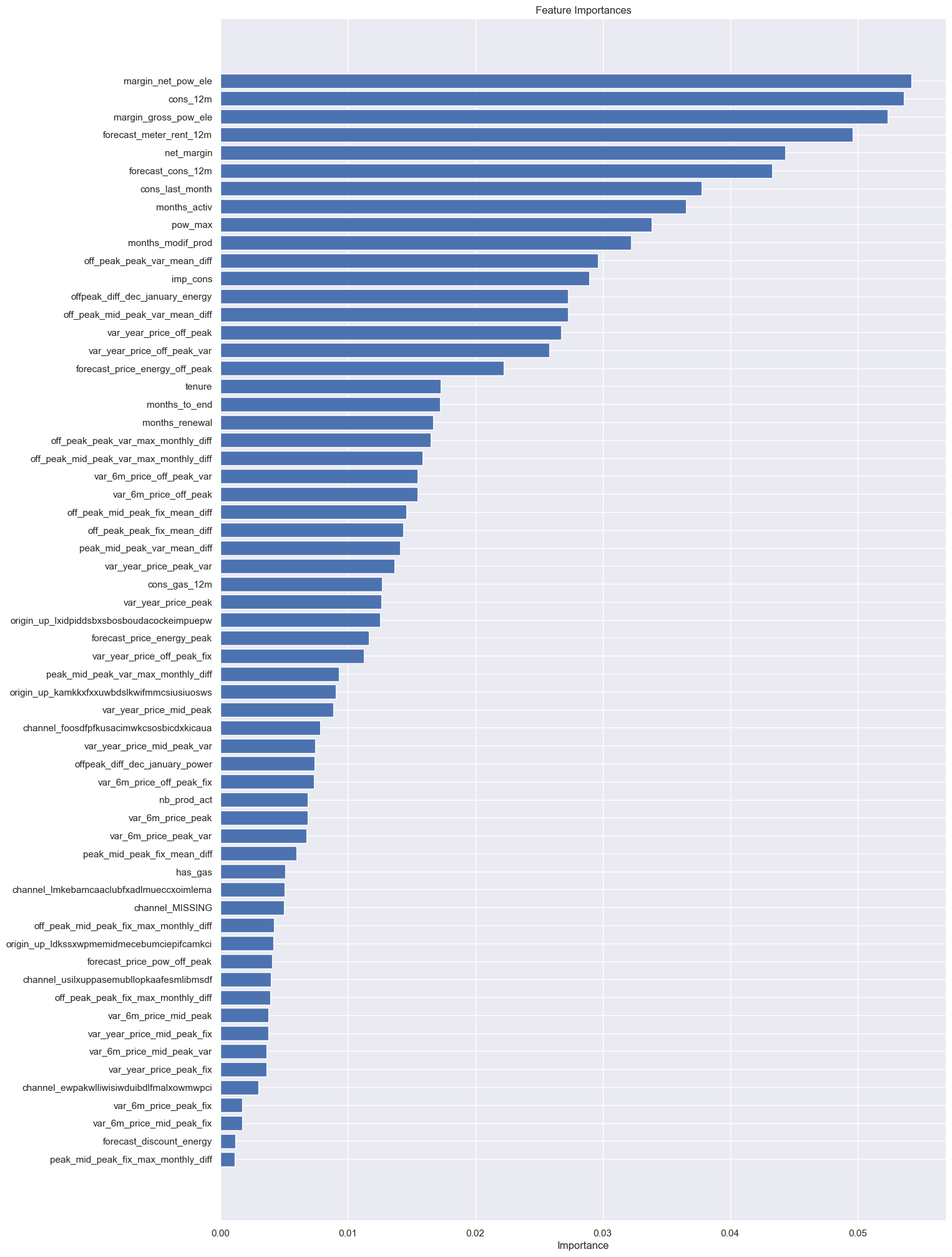
A simple way of understanding the results of a model is to look at feature importances. Feature importances indicate the importance of a feature within the predictive model, there are several ways to calculate feature importance, but with the Random Forest classifier, we’re able to extract feature importances using the built-in method on the trained model. In the Random Forest case, the feature importance represents the number of times each feature is used for splitting across all trees.
feature_importances = pd.DataFrame({
    'features': X_train.columns,
    'importance': model.best_estimator_.feature_importances_
}).sort_values(by='importance', ascending=True).reset_index()

plt.figure(figsize=(15, 25))
plt.title('Feature Importances')
plt.barh(range(len(feature_importances)), feature_importances['importance'], color='b', align='center')
plt.yticks(range(len(feature_importances)), feature_importances['features'])
plt.xlabel('Importance')
plt.show()
Complete modelling and evaluation script -
Insights & Recommendations
Churn is high in SME with 9.7% across 14606 customers for PowerCo The model was able to predict churn but Yearly consumption, forecasted consumption and net margin were important. However the price sensitivity features are scattered around and were not a main driver for churn. More modelling, fine tuning of features and inclusion of more variables is required to potentially improve the model.
A discount strategy of 20% would be effective but only if targeted appropriately. We recommended offering discount to only to high value customers with high churn probability.